
Root-me 1 is a nice place to learn different aspect of cyber-security.
Whithin the information security field, there is a steganography, which is the art of hiding information without being noticed. One principle in cryptography, the Kerckhoff’s principle stipulate that the secret when hidding a message must not be the algorithm, it must be the key. Steganography often plays against this principle. The goal is to hide a message without being discovered into genuine looking documents, like images, text, pdf, video and many others.
To solve the Root-me challenges, sometimes you need to code, sometimes you need to use the good tool to get the information. In most case, you can recode the tools yourself. It takes time, but its feasible. It is nice to learn working with the different encoding format (base64, ASCII, binary, …) and to learn a few nice algorithms.
However, sometimes you can’t, even with the best imagination possible. There is one steganography challenge where I was stuck, tried many things, none worked. I asked for help, and “there is a tool on Github which solve the challenge in a second”.
This tool is plainsight 2. Because I spent a lot of time trying solutions, I wanted to know why I failed to code it, and started to look at the code.
Maybe the code was “efficient”, but it was barrely readable:
if ... elif ... elif ...After some time, I finally understood how it worked. Because of the difficulty to understand how it worked, I decided to recode it.
It was a python2 script.
The first thing I did is to convert it to python3, by changing the syntax of some updated operators like xrange.
Despite the few changes, scripts were no more compatible.
I found the issue, and this one cannot be patched (I got troubles to get the information necessary to fill the gap).
Therefore, in this post, I will:
plainsight worksYou can jump to the section of interest directly:
Plainsight combines two concepts together:
We will detail these two concepts in the following subsections.
Huffman coding (encoding a message using Huffman trees) is a method to compress a signal to transmit. Because some letters, some words occurs more frequently than others, the distribution asymmetry is exploited to encode and transmit a message with less symbols.
Computers speak in bits. They only use 0 and 1 to do, store, make things.
To encode our 26 alphabet letters, one solution is to encode it over 5 consecutives bits.
With these 5 bits, we can encode at most \(2^5=32\) words, which is sufficient for our 26 letters.
For instance, we would code A as 00000, B as 00001, and Z as 11001.
We would have 6 unused codes like 11011 or 11111, which is one source of inefficiency.
In this previous example, we used letters because we can recreate all possible words using them.
However, if we have a limited corpus of words, we can decide to encode them directly.
If you play the game “paper, rock, scissors”, you can code paper as 00, rock as 01, and cisors as 10.
This will reduce drastically the size of the transmitted signal, as a four-letter words (which would require \(8 \times 4\) bits in ASCII) is encoded using only two bits.
Knowing the set of symbol used is a first start to compress a signal.
It is convenient to compute the size of the resulting message, which is #symbol x CodeLength.
The compression efficiency can be improved by playing on code length. The main idea is that frequent items would get shorter codes, while infrequent ones get longer codes. As all codes would not have the same length, it means that we can only decode sequentially the message. We cannot use multiple thread, one that would process the first half, and another the second half because maybe the signal bit streal will be cut in the middle of a symbol.
If we have multiple codes of different length, we would like the reading to be non-ambiguous.
This is where the magic of trees occurs.
They allows to represent code and to verify that one code is not the suffix of another.
For instance, if the code 01 exists, then we have guarantees that 011 and 010 do not exist.
To find the codes, we need to build a Huffman tree.
Suppose there is a list of symbols \(S = \{s\}\) with respective frequencies \(\{f_s\}\). At the start, we create \(|S|\) unlinked nodes, one for each symbol, with weight \(w_s = f_s\)
To construct the tree, we loop over these instructions’ set until there is one node left:
n_a and n_b, two nodes with the lowest weight (w_a < w_b)n_c with weight w_a + w_b, with left child n_a and right child n_b.n_a and n_b from the working set of available and add n_c to the set.Now, the tree is built, where all the symbols we want to encode are the leaves of the tree.
To obtain the code associated to each symbol, you need to travel through the tree. To find the code corresponding to a symbol, you start from the root and move to your word using the single existing path. When you move through an edge, you update your code:
0 to the current code1 to the current codeThe order doesn’t really matter in terms of encoding length.
We could assign 1 to the left direction and 0 to the right one.
It is even possible to flip it at random: sometimes left direction is 1, sometimes 0.
When compressing a file with a Huffman Tree, there would be a prelude saying “01 is xx, 00 is yy, and 1 is zz”.
But when the tree is not directly shared (for instance, you say you learned frequencies on corpus xx), the receiver cannot guess what is your encoding, unless you follow the conventions.
Here is a simple python implementation.
Here, the inputs are the frequencies. The result reffers to the index into the input list.
To get the code of symbol \(s_i = S[i]\) with frequency \(f_i\), we just need to look at the output at index \(i\).
def get_huffman_codes(freqs):
  """
  Compute the Huffman codes corresponding to the given word frequencies.

  :param freqs: a list of frequencies (non ordered)
  :rparam: the list of binary codes associated to each frequency
  """
  lst = sorted(map(lambda x: (x[1], [x[0]]), enumerate(freqs)))

  # Initialize code words
  dic_code = dict([(ID, '') for ID, _ in enumerate(lst)])

  while len(lst) > 1:
      # The first one has the lowest frequency, which would get a 1
      m1, m0 = lst[0], lst[1]

      # Iterate over all the IDs, and happend a 1 or a 0
      for c in m1[1]:
          dic_code[c] = "1" + dic_code[c]
      for c in m0[1]:
          dic_code[c] = "0" + dic_code[c]

      f_tot  = m1[0] + m0[0]
      ID_tot = m1[1] + m0[1] # List concatenation

      # For very large list of words, this is not optimal
      # It does the job for small inputs.
      lst = sorted([(f_tot, ID_tot)] + lst[2:])

return list(dic_code.values())Let’s look at English letters frequencies3.
The first most frequent letters are listed in this table:
| Letter | Freq |
|---|---|
| E | 11.2% |
| A | 8.5 % |
| R | 7.6 % |
| I | 7.5 % |
| O | 7.1 % |
| T | 7.0 % |
| N | 6.7 % |
The corresponding Huffman tree is:
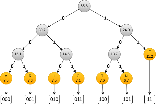
You can see that only E get the shortest code.
This is because the differences between frequencies are not very large.
Nonetheless, compare to a fixed 3 bits encoding, we save 1 bit 11% of the time.
The obtained code depends on the alphabet size and the frequencies. If we look at the corresponding trees for the top-6 and top-5, we get:
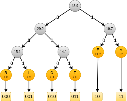
and
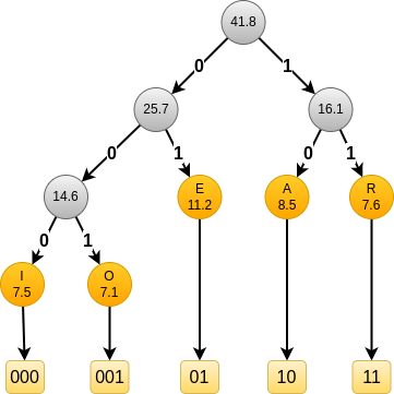
In all these cases, E always get a short code of length 2.
Depending on the case, it gets code 01, 10 and 11.
To decode a message, we need to know what are the corresponding codes.
If you want to know more about Huffman Trees, you can have a look at:
There are multiple approaches to generate texts. The first one is to study language letters’ frequency. The results are not very good and we get a soup of letters, because we look at a very narrow quantity.
To improve likelihood, the idea is to look letters over a window.
If you look over a window of size two, you will learn which letters can follow each other.
You will learn that a-a never occurs, and that w-h is very frequent.
The generated text will be made of words that seem to belong to the current language, but most of them do not exists.
You can increase the window, to three or more. The larger the better.
Instead of looking at letters, you can consider words directly. When decomposing a sentence into words, a \(n\)-grams is a tuple of \(n\) successive words.
For instance, The cat is grey is equivalent to the list [The, cat, is, grey].
There are three possible bi-grams:
(The, cat)(cat, is)(is, grey)and two possible tri-grams:
(The, cat, is)(cat, is, grey)and one 4-grams.
To generate a text that looks natural, it must have properties similar to regular text.
The first quantity to look at is word frequency.
To generate a text, we cannot pick at random words from a dictionary. Words tends to be distributed according to a power law or Zipf law. In other words, a few words are highly frequent while most of the rest almost never occur. If you pick words at random in a dictionary, it is very likely that you almost never use those words.
Next, we have grammar. There are rules that governs how words are located in a sentence. Frequencies are not sufficient. Coding grammar rules is possible, but time consuming. To avoid this coding, we can instead look at \(n\)-grams. If we have a large corpus, we know what are the valid words following a sequence.
If \(P(w_k | w_0, w_1, ..., w_{k-1}) > 0\), then the word \(w_k\) is a candidate. If \(k\) is large, we often have enough context to select a word that is valid according to grammar rules.
Suppose our corpus is made of:
The cat is greyThe cat is sleepingThe dog is black(The, dog) + (dog, is) + (is, grey) gives The dog is grey, which is a valid sentence in our language.
However, is our corpus is:
The fire is hotThe ice is blueThe ice is hot and The fire is blue are valid in terms of grammar, but wrong in terms of truth.
Using large n-grams plus a large corpus allow to avoid grammar error and aberrant sentences.
To construct a text with \(n\)-grams, you use the \(n-1\) previous words to find the \(n^{iest}\) words.
This is in this second case where Huffman trees are used.
Given a context w_1, w_2, ..., w_(n-1), you have k options w_(o1), w_(o2), ..., w_(ok), each with a particular frequency.
Using an Huffman tree for this particular context, you can associate to each of these k words w_ox a binary code word.
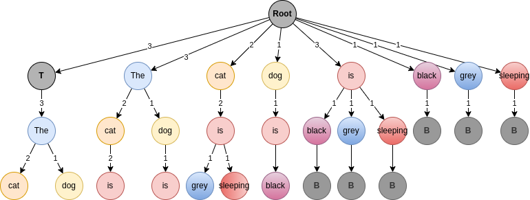
w_nTaking back our cats and dog example, we get the following tree for bi-grams.
We added symbols TOP and BOTTOM to mark the start or end of a sentence.
This allows to reset the context memory.
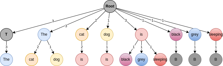
The goal is to encode 011010.
At the start, we know that we must start a sentence.
We follow the path Root -> TOP.
Here, there is a single choice, so no bit can be encoded.
Because we use bi-gram, we have one word of memory, i.e. C=[The].
We follow the path Root -> The.
Here, we have two options: cat with code 0 and dog with code 1 (because cat is more frequent than dog).
Because our first bit is 0, we select cat.
Now, the current message is M=[The, cat], the context C=[cat], and the leftover bits 11010.
We follow the path Root -> cat. Same than with The, one single choice.
We follow the path Root -> is. Here, three choices.
Because they all have the same frequency, we select the lexicographic order
(we have code 00 for grey, 01 for black, and 1 for sleeping).
We select sleeping,
so now, the current message is M=[The, cat, is, sleeping], the context C=[sleeping], and the leftover bits 1010.
Now, single choice, ending the sentence.
We start back with TOP.
Repeating the process, we have:
The cat is sleeping. The dog + 010The cat is sleeping. The dog is black + 0The cat is sleeping. The dog is black. The cat + ``Decoding is as easy as encoding. If I just summarize context, bits recovered and leftover, we have:
C=[TOP], B="", M="The cat is sleeping BOT TOP The dog is black BOT TOP The cat"C=[The], B="", M="cat is sleeping BOT TOP The dog is black BOT TOP The cat"C=[cat], B="0", M="is sleeping BOT TOP The dog is black BOT TOP The cat"C=[is], B="0", M="sleeping BOT TOP The dog is black BOT TOP The cat"C=[sleeping], B="01", M=" BOT TOP The dog is black BOT TOP The cat"C=[BOT], B="01", M="TOP The dog is black BOT TOP The cat"C=[TOP], B="01", M="The dog is black BOT TOP The cat"C=[The], B="01", M="dog is black BOT TOP The cat"C=[dog], B="011", M="is black BOT TOP The cat"C=[is], B="011", M=" black BOT TOP The cat"C=[black], B="01101", M="BOT TOP The cat"C=[BOT], B="01101", M="TOP The cat"C=[TOP], B="01101", M="The cat"C=[The], B="01101", M="cat"C=[cat], B="011010", M=""And we recovered our initial message.
A previous implementation of plainsight can be found on Github.
At the start, we just wanted to modify some operators so the python2 script could be used with python3.
Changing the xrange into range was quite easy.
However, we got a problem:
In both implementation, the \(n\)-grams trees is coded using dictionaries.
However, python2 and python3 dictionaries are not implemented the same way.
Especially concerning the key sorting algorithm:
python2, dictionary keys are sorted according to a specific hash function.python3, dictionary keys are sorted according to the arrival. I.e., if dog is added before cat, then dog is the first key, and cat the second.Look at these two examples:
With python2:
dic = {"dog": 1, "cat": 3, "frog":5}
print(dic)
> {'dog': 1, 'frog': 5, 'cat': 3}
With python3:
dic = {"dog": 1, "cat": 3, "frog":5}
print(dic)
> {"dog": 1, "cat": 3, "frog":5}
This creates the incompatibility. The two codes are not compatible. Nevertheless, our implementation has a deterministic sorting: first by frequency and next according to the lexicographic order, making it compatible with other implementations.
plainsight I doesn’t use Huffman trees.
Instead, when a choice can be made to finish a \(n\)-grams, it encodes all solution with a fixed length code (depending of the \(n-1\) previous words).
If \(W\) is the set of possible words following the current \(n-1\)-gram, with \(|W|=s > 1\)
then it exist a \(k_s\) such as \(2^{k_s} \leq s < 2^{k_s+1}\).
The \(2^{k_s}\) most frequent words would get an associated binary code.
As an example, if we have \(7\) candidates, \(k=2\) therefore only \(4\) of these \(7\) candidates can be used to encode bits.
The most frequent one would get the code 00, the next 01, the third 10 and the last 11.
Because some words are not selected for coding, the richness of the generated text will be smaller. This is not a big problem as the code will always run and always be able to encode a message.
If only \(2^{k_s}\) over the \(s\) items are coding, it doesn’t mean that the \(s-2^{k_s}\) last items are discarded. The intermediate nodes of the tree (not root, not leaf) are possible paths.
Look at the following figure, which represents the 3-grams of a synthetic corpus:
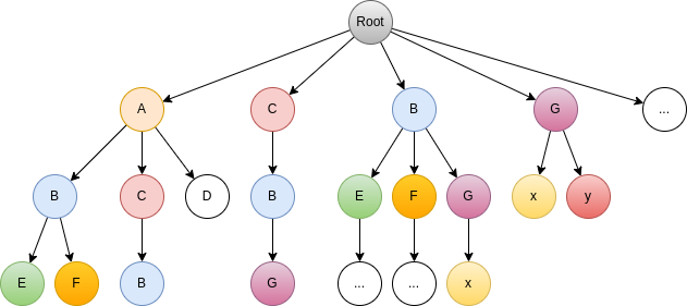
This is the state when we have added all the \(n\)-grams to the tree. The nodes are sorted from left to right by decreasing frequency.
If we look at node G, it can be access using the path Root -> C -> B -> G.
The only possible path after removing C from the context is Root -> B -> G -> x
If we prune the tree, we get:
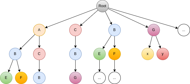
where this last path doesn’t exist anymore. A true pruning only exists at the leaf level, where it is never possible to select one of the low frequency items.
If you select a small tree depth (2 or 3), the text wouldn’t look very natural.
In the other hand, if the depth is too large, the n-grams possibilities are less numerous.
As a consequence:
which leads in the end to very large messages. For instance, if you look at the tree of depth \(3\):
you can see that there are 2 final forks: (TOP, The) -> (cat|dog) and (cat, is) -> (grey|sleeping)
To consume the bits of the message to hide, they can only be encoded using these two transitions.
There are three possible sentences:
The cat is grey which encodes 00The cat is sleeping which encodes 01The dog is black which encodes 1On average, we consume on average \(1.6\) bits per sentence, which is smaller value than with a tree of depth 2, where each sentence could encode 2 to three bits (previous example).
If you have one byte to hide (one ASCII character), you need at min 4 sentences of 4 words.
If you use very large \(n\)-grams, the beginning of the sentence will often condition all the following words. You will always be able to encode your message, but this will take a lot amount of space.
The \(n\)-gram size must be selected according to the corpus size (and corpus quality).
Over the Sherlock Holmes corpus and depth=5, we found:
ah jack she said i have just been in to see if i can be of any assistance to our new neighbors why do you look at me like that jack you are not angry with meah jack she said i have just been in to see if i could catch a glimpse of the strange face which had looked out at me on the day before as i stood there imagine my surprise mr holmes when the door suddenly opened and my wife walked outYou can see how similar are the two sentence beginning.
Running it with depth=3:
ah jack she criedah jack she cried with a startled faceah jack she cried trust me jack she said i at last however there came an overwhelming desire to see her slinking into her own husband spoke to her however before i ran into the other side of the gnu fdl 3ah jack she cried i swear that this mystery comes to an end from now you are surprised said she and i had to choose between you and in my direction and her footsteps coming up the lane but i did not even knock when i left her in peace having no success she goes again next morning and her dutyWith a smaller depth, said is no more used.
In the corpus jack she cried might occurs more frequently than jack she said.
For depth=5, ah jack she cried never occurs.
In both version, bits can be hidden whenever there is at least two choices in the current context node of the tree.
In the first version, only \(2^k\) of the \(n\) children nodes can be selected. This reduce the diversity of the possible messages that can be constructed. Nevertheless, assigning the code are much faster in this version, as we only need to rank nodes by frequency.
In the second version, any of the children can be selected. Infrequent words encode more bits than frequent ones. But it is unlikely that a large code word match exactly the current bit string to encode. One of the disadvantage of this method is the stability with regards to the corpus. If some sentences are discarded from the corpus, the vocabulary set may change and code words reassigned.
The efficiency of a steganographic system correspond to the number of bits encoded versus the size of the encoded message. Because we use words to encode bits, the ratio is low. Because there are trivial transition, this add words with no encoding power to the message. Therefore this is quite inefficient.
The second aspect for steganographic evaluation is the detection threshold.
Compare to cryptographic systems, plainsight is a kind of secret-key steganographic system, as without the corpus and the depth, you cannot recover the message.
In this implementation, the word transition encodes the bits. It is possible to work at different levels:
Instead of text, you can work on graphs. According to a ranking/scoring function, you order the neighborhood of your current nodes / current path, and jump to a valid neighbors. With this approach, you can generate:
You can also work on a fixed set of elements, like paper, rock, scissors, create images, time series … There are many other ways to play with this type of encoding method.
In this post, we explained how plainsight work to generate genuine-looking hiding messages. When reading and testing the initial code, I discovered that the result of the previous version was language dependent, preventing the compatibility with other implementations. This compatibility problem was linked to the way keys are sorted within dictinaries. In this new version, the sorting is no more language deterministic, which make us less dependent from a single tool. We also simplified drastically the code, getting the same number of lines of code while adding documentation. You can find the code on Github 6.
>> You can subscribe to my mailing list here for a monthly update. <<