<< Go back to Tech

Political blogosphere visualization Data

Anonymous on my blog ? Do you think ? If I connect to the other, someone can learn about my opinion from my neighbors. Here is an example on the US political blogosphere of 2004.

Introduction

Graphs are everywhere.

Communication and social networks are two good examples.

Your message might be encrypted, but the intent is not ! Which community you belong to can be easily recovered by graph analysis.

Here I show a simple example using the polblog dataset. ¹

Dataset

In the Political Blog dataset ¹, you have several information:

blogs name;
blogs outgoing links;
blogs political orientation (left or right).

It was collected for the 2004 US presidential election, and there are about 1500 blogs in it.

Visualization

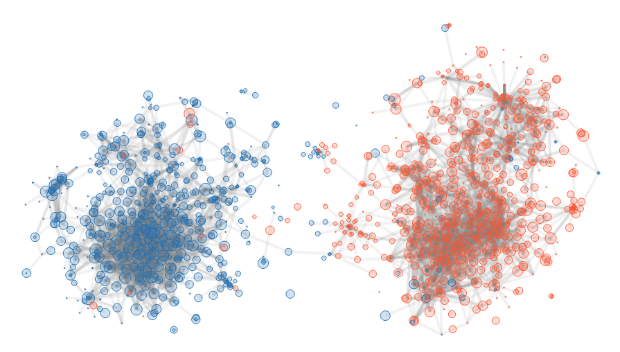
The illustration is straightforward: two distinctive groups. There are some outliers, blue points in red cluster and vice-versa. This is due to the fact that we study links, but we have no way to weight them. A blog trying to criticize the opposition is like a blog defending them because there is no way to weight positively or negatively a link.

Political Blogosphere

Processing

In the following, we explain how we get this result.

Notation

We have a directed graph $G=(V, E)$. $V$ represents the blogs, while $E$ the link from one blog to another.

We define the outgoing $\mathcal{N}$ and incoming neighborhood $\mathcal{N}^{-1}$ as:

\[\mathcal{N}(u) = \{v | (u, v) \in E\}\] \[\mathcal{N}^{-1}(u) = \{v | (v, u) \in E\}\]

And $\|\mathcal{N}(u)\|$ represents the number of neighbors $u$ can directly reach.

Representation

Usually, a graph is represented by a list of tuples, for instance:

[
  [1, 2],
  [1, 3],
  [3, 4]
]

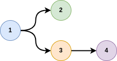
where here, node 1 is connected to node 2 and 3, and 3 to node 4. This representation is efficient in terms of memory consumption. However, this is unpractical for making calculation. We need to represent this as a binary matrix:

[
  [0, 1, 1, 0],
  [0, 0, 0, 0],
  [0, 0, 0, 1],
  [0, 0, 0, 0],
]

As you can see, the matrix is very sparse at it contains a lots of zeros.

This matrix is also called the adjacency matrix, which is denoted $A$ in the following.

Pruning: Getting the Largest Connected Component

When getting a graph, usually it is made of several disconnected components. Small graphs are difficult to analyse, because there is no information. Identification of the connected components is easy, and can be done with the following function, expecting a graph represented by a python dictionnary { "my_node": [list of connected nodes]}

def get_connected_components(dic_c):
    """Find connected components. Sort them by decreasing size

    :param dic_c: dic of relationships
    :rparam: list of [list of connected items]
    """
    # Initial color of a node

    dic_color = dict([(c, idx) for idx, c in enumerate(dic_c)])
    dic_group = dict([(idx, [c]) for idx, c in enumerate(dic_c)])

    for idx, (c, lsi) in enumerate(dic_c.items()):

        # Get the lit of possible colors
        colors = set(map(lambda x: dic_color[x], [c] + lsi))

        if len(colors) == 1:
            # all nodes have belongs to the same group
            continue

        # Sort color by count. Use the "best color" to replace all
        colors = sorted(colors, key=lambda x: len(dic_group[x]), reverse=True)
        col = colors[0]

        for col_i in colors[1:]:
            # Add colored node to same group
            dic_group[col].extend(dic_group[col_i])
            # Change color of nodes
            for s in dic_group[col_i]:
                dic_color[s] = col

            # remove group
            del(dic_group[col_i])

    return sorted(dic_group.values(), key=lambda x: len(x), reverse=True)

In the current case, the largest group has more than $1,000$ nodes, and the second largest has … only $2$ nodes. The decision to discard small groups is easy.

Describing a Node

Graphs are difficult to process compared to tabular data because:

Data structure is completely different, there are no “features”
Nodes are described by their neighborhood
Adjacency matrix is very sparse

To compare two nodes in a tabular way, we could compare node description from the adjacency matrix $A$. However, this matrix is very sparse, and the overlap between two nodes is frequently $0$.

To overcome the problem, the idea is to look at distant neighbors. Adjacency matrix represent the neighbors at distance $1$. Instead, we can look at neighborhood up to distance $d$. This is the idea of random walk: you start from one node, and you “jump” with some probability to neighborhood nodes. The more neighbors there are, the lowest the probability.

To compute the probability to jump to a node up to distance $d$, we first need to construct the transition matrix $T$ such as:

$T_{i, j} = \frac{A_{i, j}}{deg(i)}$.

With this transition matrix, we compute different diffusion location:

\[C^{i} = \mathbb{I} \left(T^{T}\right)^i\]

If you perform many steps, you are likely to converge to a stable matrix. Here, this stable state is of no interest for our case.

We compute a weight matrix $W$ such as:

\[W_{i, j} = \sum_{k=0}^d C^{(k)}_{i, j}\]

In our case, $d = 4$ is enough, and enable to pay attention to neighborhood up to distance $4$.

We could have chosen another value for $d$. However, if $d$ is too low, then the vector describing a node would be very sparse as very few neighbors would have been reached. If $d$ is too large, then we would reach a stable state, and many items would share this same state. Therefore, it would be difficult to identify the difference between nodes. $4$ is a good number, but it depends on the case. For a smaller average degree, a larger number would be necessary. For a highly connected graph, a smaller one would be enough.

Comparing Two Nodes

As we have weights, the cosine similarity is great to compare two nodes:

\[S(u, v) = \frac{\mathbf{w}^u \mathbf{w}^v}{\|\mathbf{w}^u\|\|\mathbf{w}^v\|}= \frac{\sum_{i \in \mathcal{N}} w^u_i w^v_i}{\sqrt{(\sum_{i \in \mathcal{N}} w^u_i )(\sum_{i \in \mathcal{N}} w^v_i )}}\]

Or shortly:

\[S(u, v) = \frac{\mathbf{w}_u \mathbf{w}_v^T}{\sqrt{\|\mathbf{w}_u\| \|\mathbf{w}_v\|}}\]

with:

\[\|\mathbf{x}\| = \sum_{i} x_i^2\]

This return a value in $[0, 1]$, where a value close to $1$ means that the two nodes are very close.

From Similarity to Distance

Most embedding algorithms such as $t$-SNE rely on distance between items. Here, we have similarity. To convert similarity into distance, we transform the matrix by using inverse.

\[D = \frac{1}{S + \epsilon} - \frac{1}{1+\epsilon}\]

The $\epsilon$ is a small value ($\approx 10^{-5}$) avoiding the division by zero. The second term enables to get the best minimal value equal to zero.

Building an Embedding

We use $t$-SNE ² for this purpose. $t$-SNE is an embedding algorithm. It is used to represent high dimensional data into a low dimensional space, where it is easy to visualize the data.

The code for this operation is very simple, thanks to the nice sklearn python library.

from sklearn.manifold import TSNE

Y = TSNE(perplexity=30, metric="precomputed", square_distances=True).fit_transform(D)

The TSNE() method can take as input a distance matrix when the argument metric is set to precomputed. Otherwise, it would consider $D$ as a vector where distance must be computed …

The input of this algorithm is a set of vectors or a distance matrix. Here we “convert” the similarities we obtained by inversion to get a “distance”. You can see the full details on ArXiv ³.